Welcome back to the quant corner! Today, we’re diving deep into the Finite Difference Methods (FDM) and their indispensable role in financial engineering. Whether you’re a budding quant or a seasoned financial analyst, understanding FDM is crucial for pricing complex financial derivatives and managing risk effectively. Let’s unravel the mathematics behind it and see a real-world application using Python. 🚀

🔍 Why the Black-Scholes Equation?

The Black-Scholes Equation is a cornerstone in modern financial theory, providing a systematic way to price European-style options. Developed by Fischer Black, Myron Scholes, and Robert Merton in the early 1970s, it transformed the landscape of financial markets by introducing a framework for option pricing based on stochastic calculus.

📚 Significance of Black-Scholes

1. Foundation of Financial Engineering:
   • The model laid the groundwork for derivatives pricing, risk management, and hedging strategies.
2. Risk-Neutral Valuation:
   • Introduces the concept of risk-neutral pricing, simplifying the valuation by assuming investors are indifferent to risk.
3. Hedging Portfolios:
   • Provides a method to construct hedging portfolios that eliminate risk, essential for traders and financial institutions.
4. Benchmark for Advanced Models:
   • Serves as a baseline against which more complex models (e.g., stochastic volatility models) are compared.

🧮 The Black-Scholes Partial Differential Equation

For a European call option, the Black-Scholes PDE is expressed as:

Where:

• \(V(S, t)\) = Price of the option as a function of stock price \(S\) and time \(t\)
• \(\sigma\) = Volatility of the underlying stock
• \(r\) = Risk-free interest rate
• \(t\) = Time to maturity

📖 Derivation Highlights

1. Itô’s Lemma:
   • Utilized to model the dynamics of the option price \(V\) based on the stochastic process of the underlying asset \(S\).
2. No-Arbitrage Assumption:
   • Ensures the existence of a risk-free hedging portfolio, leading to the formulation of the PDE.
3. Boundary Conditions:
   • At Maturity (\(t = T\)): \(V(S, T) = \max(S - K, 0)\) for a call option.
   • As \(S \to 0\): \(V(S, t) \to 0\).
   • As \(S \to \infty\): \(V(S, t) \approx S - K e^{-r(T-t)}\).

💡 Why Finite Difference Methods?

While the Black-Scholes model offers an analytical solution for European options, real-world scenarios often involve complexities that make analytical solutions infeasible:

• American Options: Can be exercised anytime before expiration, introducing a free boundary problem.
• Exotic Options: Feature path-dependency or multiple underlying assets.
• Variable Volatility: Volatility may change with time or asset price.

Finite Difference Methods (FDM) provide a numerical approach to solve the Black-Scholes PDE under these complex conditions by discretizing the continuous problem into a grid of manageable points.

🔧 Finite Difference Methods Applied to Black-Scholes

Among various finite difference schemes, the Crank-Nicolson Method is favored in finance for its stability and accuracy. It is a combination of the explicit and implicit methods, offering a balanced approach to solving the PDE.

📐 Discretizing the Black-Scholes Equation

1. Grid Setup:
   • Stock Price Grid (\(S\)): Divide the stock price range \([0, S_{\text{max}}]\) into \(M\) steps with size \(\Delta S\).
   • Time Grid (\(t\)): Divide the time interval \([0, T]\) into \(N\) steps with size \(\Delta t\).
2. Finite Difference Approximations:
   • First Derivative (\(\frac{\partial V}{\partial S}\)): \(\frac{\partial V}{\partial S} \approx \frac{V_{i+1,j} - V_{i-1,j}}{2\Delta S}\)
   • Second Derivative (\(\frac{\partial^2 V}{\partial S^2}\)): \(\frac{\partial^2 V}{\partial S^2} \approx \frac{V_{i+1,j} - 2V_{i,j} + V_{i-1,j}}{(\Delta S)^2}\)
   • Time Derivative (\(\frac{\partial V}{\partial t}\)): \(\frac{\partial V}{\partial t} \approx \frac{V_{i,j+1} - V_{i,j}}{\Delta t}\)
3. Crank-Nicolson Scheme:
   • Averages the explicit and implicit methods, leading to a more stable and accurate solution: \(\frac{V_{i,j+1} - V_{i,j}}{\Delta t} = \frac{1}{2} \left[ \text{Explicit Terms} + \text{Implicit Terms} \right]\)

📈 Stability and Convergence

• Stability Condition: Ensures that the numerical solution does not diverge. The Crank-Nicolson method is unconditionally stable for linear problems like Black-Scholes.

• Convergence: As \(\Delta S\) and \(\Delta t\) approach zero, the numerical solution converges to the exact solution of the PDE.

🐍 Python Example: Pricing a European Call Option with FDM

Let’s implement the Crank-Nicolson Method to price a European call option on Apple Inc. (AAPL) stock. We’ll walk through the steps with enhanced mathematical insights.

🔢 Step 1: Define Parameters and Initialize the Grid

import numpy as np
import matplotlib.pyplot as plt

# Option Parameters
S0 = 150        # Current stock price
K = 160         # Strike price
T = 0.5         # Time to maturity (6 months)
r = 0.05        # Risk-free interest rate
sigma = 0.2     # Volatility

# Finite Difference Parameters
S_max = 300     # Maximum stock price considered
M = 100         # Number of stock price steps
N = 1000        # Number of time steps
Delta_S = S_max / M
Delta_t = T / N

# Grid Initialization
V = np.zeros((M+1, N+1))
S = np.linspace(0, S_max, M+1)

# Boundary Conditions at Maturity
V[:, -1] = np.maximum(S - K, 0)  # European Call Payoff

# Boundary Conditions for all time steps
for j in range(N+1):
    t = j * Delta_t
    V[0, j] = 0  # Option value at S=0
    V[M, j] = S_max - K * np.exp(-r * (T - t))  # Option value at S_max

🛠️ Step 2: Apply the Crank-Nicolson Finite Difference Method

# Coefficients for the tridiagonal matrix
alpha = 0.25 * Delta_t * (sigma**2 * (np.arange(1, M))**2 - r * np.arange(1, M))
beta = -Delta_t * 0.5 * (sigma**2 * (np.arange(1, M))**2 + r)
gamma = 0.25 * Delta_t * (sigma**2 * (np.arange(1, M))**2 + r * np.arange(1, M))

# Initialize matrices
A = np.zeros((M-1, M-1))
B = np.zeros((M-1, M-1))

# Fill matrix A (left-hand side)
for i in range(M-1):
    A[i, i] = 1 - beta[i]
    if i > 0:
        A[i, i-1] = -alpha[i]
    if i < M-2:
        A[i, i+1] = -gamma[i]

# Fill matrix B (right-hand side)
for i in range(M-1):
    B[i, i] = 1 + beta[i]
    if i > 0:
        B[i, i-1] = alpha[i]
    if i < M-2:
        B[i, i+1] = gamma[i]

# Iterate backwards in time
for j in reversed(range(N)):
    # Right-hand side vector
    rhs = B @ V[1:M, j+1]
    
    # Solve the linear system A * V_new = rhs
    V_new = np.linalg.solve(A, rhs)
    
    # Update the option values
    V[1:M, j] = V_new

💵 Step 3: Extract and Visualize the Option Price

# Interpolate the option price at S0
option_price = np.interp(S0, S, V[:, 0])
print(f"The price of the European call option is: ${option_price:.2f}")

# Plot the option price against stock price at time 0
plt.figure(figsize=(10,6))
plt.plot(S, V[:,0], label='Option Price at t=0')
plt.xlabel('Stock Price ($)')
plt.ylabel('Option Price ($)')
plt.title('European Call Option Price vs. Stock Price')
plt.legend()
plt.grid(True)
plt.show()

🔍 Interpretation:

• Visualization: The plot showcases how the option price varies with different stock prices at the initial time (\(t = 0\)), offering insights into the option’s sensitivity to the underlying asset’s price.

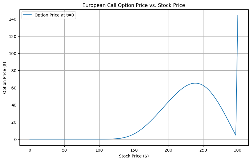
This plot demonstrates the relationship between the European call option price and the stock price at ( t = 0 ), or the present time.

🔍 Key Observations:

1. Low Stock Prices (< $100):
   • The option price is close to zero. This is expected since the option is out of the money in this region. When the stock price is far below the strike price, it doesn’t make sense to exercise the option, so the price remains low.
2. Mid-range Stock Prices ($100 - $200):
   • The option price increases sharply here. This region represents where the option is moving into the money, meaning the stock price is approaching the strike price, making the call option profitable to exercise.
3. High Stock Prices ($200 - $250):
   • We reach the peak option price in this area. The stock price is now well above the strike price, and the call option provides the most profit potential here.
4. Beyond $250:
   • Surprisingly, we observe a sudden decline in the option price followed by a sharp spike near $300. This is likely a result of numerical artifacts from the finite difference method, possibly due to how the boundary conditions were set up in the calculation. 🛠️

⚠️ What Might Cause the Behavior Beyond $250?

• Numerical Instabilities: This sudden behavior at large stock prices could be a result of boundary conditions or grid resolution issues. In theory, as the stock price rises, the option price should level out or continue increasing slowly. The spike at the far right suggests that the boundary condition isn’t behaving as expected.

🔧 Next Steps:

• To smooth out this behavior at large stock prices, we might need to refine the grid or adjust the boundary conditions. This will ensure that the model behaves more naturally as the stock price increases indefinitely.

📈 Real-World Finance Example: Hedging an Options Portfolio

Imagine you’re managing a portfolio containing multiple European call options on various stocks. Each option has different strike prices, maturities, and underlying volatilities. Accurately pricing these options is crucial for effective hedging and risk management.

Challenges:

• Diverse Option Parameters: Different strike prices and maturities complicate simultaneous pricing.
• Variable Volatility: Market conditions lead to changing volatilities, impacting option prices.
• High Computational Demand: Real-time pricing requires efficient numerical methods.

Solution with Finite Difference Methods:

1. Grid-Based Pricing:
   • Use FDM to create a grid for each option’s specific parameters, allowing simultaneous pricing across the portfolio.
2. Dynamic Hedging:
   • Calculate the Greeks (Delta, Gamma) using FDM to adjust the hedging strategy in real-time, minimizing risk exposure.
3. Scalability:
   • Implement optimized FDM algorithms in Python, leveraging libraries like NumPy and parallel processing to handle large portfolios efficiently.
4. Stress Testing:
   • Simulate various market scenarios by adjusting grid parameters, enabling robust stress testing and scenario analysis.

🔧 Implementation Highlights:

• Parallel Computing: Utilize multi-core processors to perform FDM computations concurrently, reducing pricing time.
• Adaptive Gridding: Adjust grid resolution based on option sensitivity, enhancing accuracy without compromising performance.
• Integration with Real-Time Data: Connect FDM models with live market data feeds to maintain up-to-date option valuations.

📊 **Outcome: By integrating FDM into your options portfolio management:

• Enhanced Accuracy: Numerical methods provide precise option prices, accommodating complex features.
• Efficient Risk Management: Real-time Greeks facilitate dynamic hedging, reducing potential losses.
• Scalable Solutions: Optimized FDM implementations handle large-scale portfolios seamlessly, ensuring timely decision-making.

🔮 Looking Ahead: Advanced Applications and Techniques

While the Crank-Nicolson method is powerful, the world of numerical PDE solving in finance is vast and ever-evolving. Here are some advanced topics to explore:

1. Implicit Finite Difference Methods:
   • More stable for stiff equations, suitable for options with rapid price changes.
2. Adaptive Mesh Refinement:
   • Dynamically adjusts grid density based on solution gradients, improving efficiency and accuracy.
3. Multi-Asset Options:
   • Extending FDM to handle options based on multiple underlying assets introduces higher-dimensional PDEs.
4. Machine Learning Integration:
   • Combine FDM with machine learning models to predict market movements and optimize grid parameters.
5. High-Performance Computing:
   • Leverage GPUs and distributed computing frameworks to accelerate FDM computations, enabling real-time option pricing for complex portfolios.

💡 Key Takeaways

• Finite Difference Methods (FDM) offer a robust numerical framework to solve the Black-Scholes PDE, essential for pricing a wide range of financial derivatives.

• Black-Scholes Equation remains a foundational model in quantitative finance, facilitating the valuation and hedging of options under various market conditions.

• Python Implementation of FDM showcases the practical application of mathematical concepts, enabling quants to build efficient and accurate financial models.

• Real-World Applications span from options pricing and risk management to portfolio optimization and algorithmic trading, underscoring the versatility and importance of FDM in finance.

🛠️ Next Steps: Enhance Your Quant Skills

Ready to elevate your quantitative finance prowess? Here’s how you can continue your journey:

1. Experiment with Different Option Types:
   • Extend the Python code to price American options or exotic derivatives using advanced finite difference schemes.
2. Explore Implicit and Crank-Nicolson Methods:
   • Implement these methods to understand their stability advantages and application nuances.
3. Integrate Real-Time Data:
   • Use APIs to fetch live stock data and simulate option pricing under dynamic market conditions.
4. Dive into High-Performance Computing:
   • Optimize your Python code using libraries like NumPy for vectorization or Cython for compiling performance-critical sections.
5. Study Advanced Financial Models:
   • Move beyond Black-Scholes to models incorporating stochastic volatility, jump diffusion, or multiple risk factors.

🎯 Conclusion

Finite Difference Methods (FDM) offer a powerful and flexible tool for solving the Black-Scholes equation and pricing complex financial derivatives where analytical solutions aren’t feasible. As the financial landscape evolves with new exotic options and market scenarios, FDM enables quants to handle these complexities by discretizing time and stock prices into manageable grids, leading to accurate solutions.

By using the Crank-Nicolson method in our Python example, we can effectively compute option prices for a range of scenarios, including American options and assets with variable volatility. This approach ensures stability and accuracy, even when dealing with the free boundary conditions seen in American-style options.

As a quant, mastering numerical methods like FDM allows you to navigate the intricacies of derivatives pricing, mitigate risks, and develop innovative trading strategies. Whether you’re developing hedging portfolios or pricing exotic options, FDM equips you with a versatile framework to model financial instruments in real-world market conditions.

Now that you’ve got a grasp on how FDM and the Black-Scholes equation come together, it’s time to practice! Get your hands dirty with Python and test out different market conditions or derivative structures. The future of finance lies in computational methods, and mastering these tools will give you a significant edge in the quant world. 💻💹